WGCNA run for female lncRNA. Link to code.
Step by step workflow…
- Use subsetted count matrices for males and females from the previous DESeq2 workflow
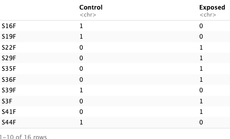
- Create metadata data frames for ID, sex, and treatment: combined, male, female
- Round count data to integers and filter out genes with row sums of 0
- 4750 lncRNAs filtered down to 4552 at this step
- pOverA setting: Basically using this to choose lncRNAs that are expressed in 50% of samples (since there are two groups control and treatment 50/50). Setting to 0 seems important since there are 2 treatments, meaning some samples would be at 0 if the lncRNA is only environmentally sensitive.
- Filtered from 4552 to 4391 assuming 1 out of all individuals expressing at least 5 counts is an appropriate metric.
- Make sure metadata frame and count matrix names match and make sure sample ID headings match the metadata frame
- Create a DESeqDataSet design from gene count matrix and labels
- log-transform the data using a variance stabilizing transforamtion (VST). This is only for visualization purposes. Essentially, this is roughly similar to putting the data on the log2 scale. It will deal with the sampling variability of low counts by calculating within-group variability (if blind=FALSE).
- Calculate the size factors of our samples. This is a rough estimate of how many reads each sample contains compared to the others. Size factors need to be less than 4.
- All size factors are less than 4
- VST transformation
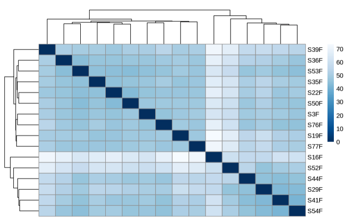
- Plot heatmap to sample distances
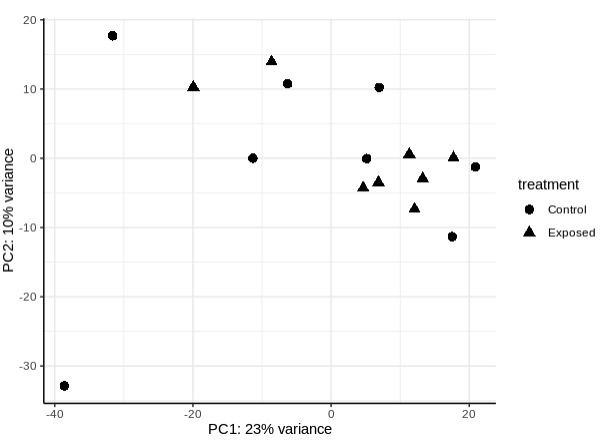
- PLot PCA by treatment
- Transpose filtered gene count matrix so gene IDs are rown and sample IDs are columns
- Check for genes and samples with too many missing values with goodSamplesGenes. There shouldn’t be any because we performed pre-filtering.
- TRUE
- Skipped outlier removal step because we expect large differences in expression since we want to capture as many lncRNAs as possible in this run.
- Choosing a soft threshold power (β). is the number to which the co-expression similarity is raised to calculate adjacency. The function pickSoftThreshold performs a network topology analysis. The user chooses a set of candidate powers.
- Use pickSoftThrshold and plot results…
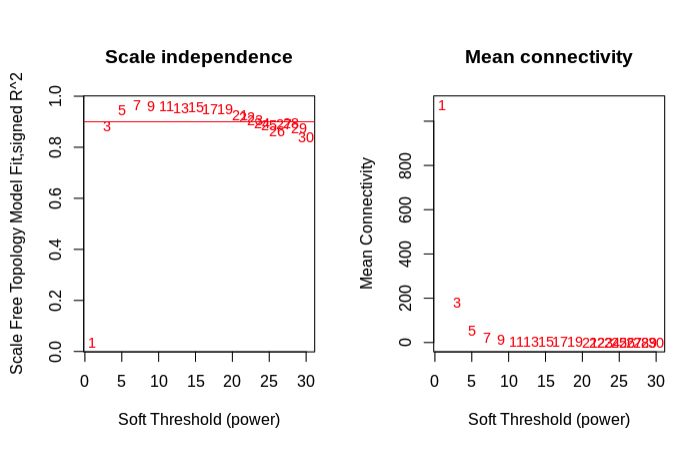
- Choose a soft threshold value at the earliest point in the curve where you see plataeu from the initial curve.
- Chose 7
- Use soft power value to calculate co-expression adjacency and create a topologinal overlap matrix of similarity.
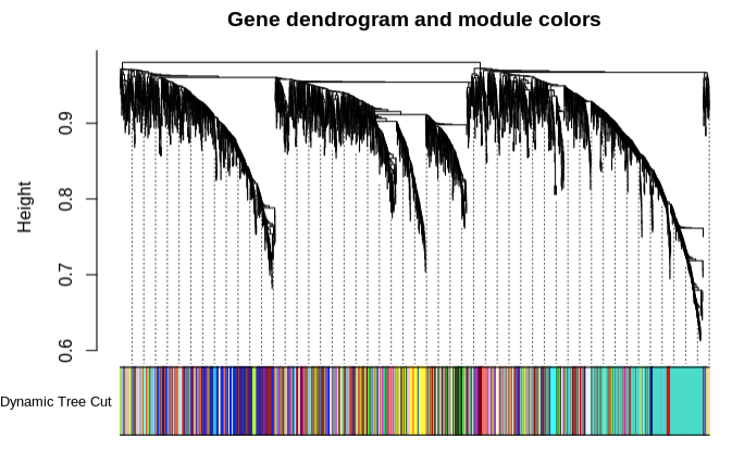
- Cluster lncRNA expression data using the topological overlap matrix (TOM)
- Form distance matrix from TOM dissimilarity and plot genet tree.
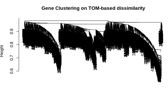
- Clustering looks good
- Identify modules of lncRNAs with similar expression patterns.
- Minimum module size set to 5
- Plot module similarity based on eigengene value
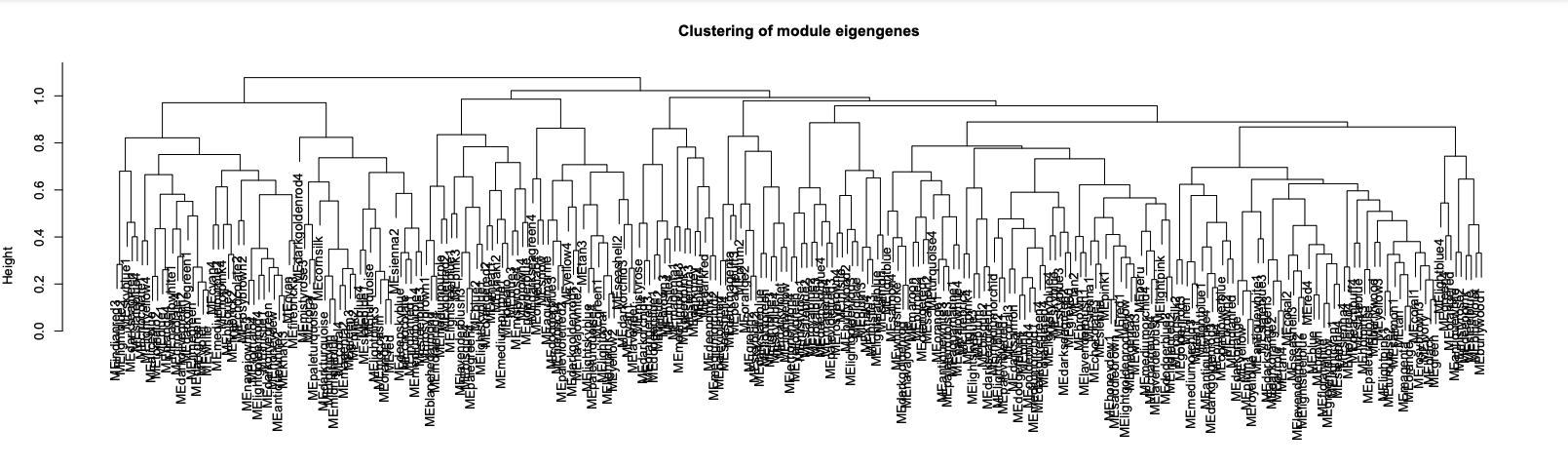
- Merge modules with >85% eigengene similarity and plot
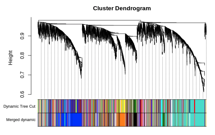
- Save merged modules
- 238 modules total
| Color | Count |
|---|---|
| aliceblue | 7 |
| antiquewhite | 7 |
| antiquewhite1 | 8 |
| antiquewhite2 | 14 |
| antiquewhite3 | 6 |
| antiquewhite4 | 11 |
| aquamarine | 5 |
| aquamarine1 | 5 |
| bisque2 | 5 |
| bisque3 | 6 |
| bisque4 | 18 |
| black | 334 |
| blanchedalmond | 6 |
| blue | 616 |
| blue1 | 7 |
| blue2 | 10 |
| blue3 | 8 |
| blue4 | 9 |
| blueviolet | 9 |
| brown1 | 8 |
| brown2 | 10 |
| brown3 | 7 |
| brown4 | 13 |
| burlywood | 6 |
| burlywood1 | 6 |
| burlywood2 | 5 |
| chartreuse4 | 5 |
| chocolate | 5 |
| chocolate1 | 6 |
| chocolate2 | 7 |
| chocolate3 | 7 |
| chocolate4 | 8 |
| coral | 9 |
| coral1 | 11 |
| coral2 | 11 |
| coral3 | 9 |
| coral4 | 15 |
| cornflowerblue | 7 |
| cornsilk | 7 |
| cornsilk2 | 6 |
| cyan | 35 |
| cyan1 | 5 |
| cyan4 | 5 |
| darkgoldenrod | 13 |
| darkgoldenrod1 | 6 |
| darkgoldenrod3 | 15 |
| darkgoldenrod4 | 7 |
| darkgreen | 58 |
| darkgrey | 21 |
| darkmagenta | 16 |
| darkolivegreen | 16 |
| darkolivegreen1 | 8 |
| darkolivegreen2 | 9 |
| darkolivegreen4 | 10 |
| darkorange | 222 |
| darkorange2 | 13 |
| darkorchid3 | 5 |
| darkorchid4 | 5 |
| darkred | 23 |
| darksalmon | 6 |
| darkseagreen | 7 |
| darkseagreen1 | 7 |
| darkseagreen2 | 8 |
| darkseagreen3 | 9 |
| darkseagreen4 | 11 |
| darkslateblue | 13 |
| darkturquoise | 22 |
| darkviolet | 10 |
| deeppink | 9 |
| deeppink1 | 8 |
| deeppink2 | 7 |
| deepskyblue | 6 |
| deepskyblue4 | 6 |
| dodgerblue1 | 5 |
| dodgerblue2 | 5 |
| dodgerblue3 | 6 |
| firebrick | 7 |
| firebrick2 | 8 |
| firebrick3 | 9 |
| firebrick4 | 10 |
| goldenrod3 | 5 |
| goldenrod4 | 10 |
| green1 | 6 |
| green2 | 7 |
| green3 | 7 |
| green4 | 8 |
| grey60 | 29 |
| honeydew | 9 |
| honeydew1 | 29 |
| hotpink3 | 5 |
| hotpink4 | 6 |
| indianred | 6 |
| indianred1 | 7 |
| indianred2 | 8 |
| indianred3 | 9 |
- Prepare trait data. Data has to be numeric, so I will substitute time_points and type for numeric values. Make a dataframe that has a column for treatment and a row for samples. This will allow for correlations between mean eigengenes and treatment.
- Correlate traits with eigengenes. Calculate correlations between ME’s and treatment. Calculate kME values (module membership).
- Generate a complex heatmap of module-trait relationships.
- heatmap found here
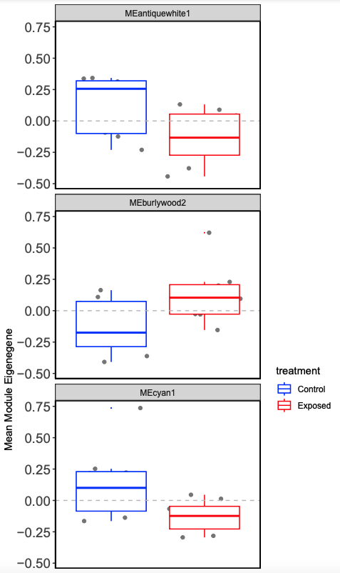
- Examine mean module eigengene values for modules of interest (those that are significant from the complex heatmap)
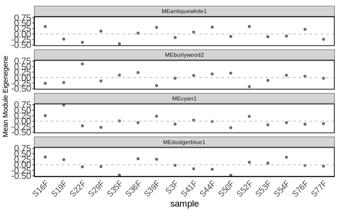
- Plot mean eigen values by treatment.
This process allows you to examine modules by treatment, so we look at expression differences more closely. Next step is to use this process on male lncRNA and then male and female mRNA to correlate between lncRNA and mRNA.